Dynasty cycle counting (penalty theory) the easy way

There are already explanations of penalty theory out there, such as this one by chaotic_iak, this one by tckmn, a section of Teal’s broader Heyawake guide, and the original Twitter thread by agnomy (in Japanese; I believe agnomy was the first person to describe penalty theory). However, none of them—that I know of—explain it in the way I find most intuitive. So I want to describe the way I think about penalty theory, in case this explanation is useful for anyone else (and to solidify my own understanding).

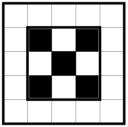
“Dynasty” describes a class of logic puzzle genres, the central example being heyawake. In a dynasty puzzle, we are asked to shade some cells in a (usually) rectangular grid such that no shaded squares are adjacent and the unshaded cells are (orthogonally) connected. Heyawake has the additional rules (1) a number in a room says how many cells in that room are shaded and (2) there is no horizontal or vertical line of unshaded cells which crosses two room boundaries. I call (2) the “heyawake rule”.

“Penalty theory” is an advanced technique for solving dynasty puzzles.¹ In brief, you use some graph theory to determine the maximum number of shaded squares that can fit subject to the dynasty constraints, which gives a bound on the number of places shaded squares can be packed inefficiently (called “penalties”). I’m not a big fan of the term “penalty”, but it’s pretty standard. I’ll call this technique cycle counting, since that’s what it’s about.

I’ve attempted to make this understandable with minimal prior knowledge, but familiarity with the basic concepts of graph theory (e.g. the terms “vertex”, “edge”, and “cycle”) is helpful. In the interest of completeness, this post is pretty long, but don’t be frightened! You should skip any parts that don’t seem useful for you, and a large portion of this post is pictures or concrete examples of working through puzzles. If you just want to understand the simplest uses of cycle counting (on the whole puzzle, with no weird shapes), you only need to read the first third or so.

If you’re just here for puzzles to practice cycle counting/penalty theory on, you can skip to the examples: 1 2 3 4 5 6 7 8.

Counting cycles

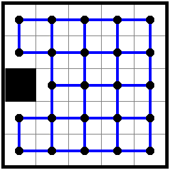
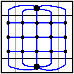
In accordance with nominative determinism, the crucial concept behind cycle counting is counting cycles in the unshaded squares. We consider the unshaded graph, whose vertices are unshaded squares and which has edges between adjacent squares. Here’s the unshaded graph (vertices black, edges blue) for an easy heyawake puzzle:²

This graph has two cycles, which I’ve drawn in red. A cycle is just a loop in the graph that ends where it starts, without any backtracking.

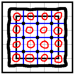
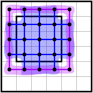
To use cycle counting, we need to count the number of cycles in the puzzle before we start shading squares. Let’s take the example of an empty 5 by 5 grid:

I’ve drawn the graph of unshaded cells, with black vertices and blue edges. How many cycles does it have? We can just count them: each small blue square is a cycle, so there are 16. More generally, each $+$-shaped intersection of grid lines corresponds to one cycle.

Fact. In an empty puzzle (with no weird topology), the number of independent cycles in the unshaded graph is the number of internal intersections of grid lines.

This is usually really easy to count: for a rectangular $r\times c$ puzzle, the intersections of grid lines are in a $(r-1)\times(c-1)$ grid, so there are $(r-1)(c-1)$ cycles.

You can think of the unshaded graph in an empty puzzle as the dual graph of the graph of grid lines (with some weirdness about the edge of the puzzle). You have to be more careful when counting cycles in puzzles with weird topology, such as holes or wraparound³.

We’re actually counting independent cycles, not all of the cycles: there are tons of cycles that are more complicated than a single square, but they can all be built by combining single squares. The number of independent cycles is the same as the number of (interior) faces of the unshaded graph.⁴ I’m going to continue saying “number of cycles” to mean the number of independent cycles.

We can also count the number of cycles just by seeing how many edges $E$ and vertices $V$ the graph has, assuming it’s connected. If $V-E=1$, then it’s a tree, so it has no cycles. Every time we add an edge, we introduce one more cycle, so the number of cycles in a connected graph is $E-V+1$. This expression⁵ is also called the reduced Euler characteristic of the graph, and is written $\bar\chi(G)$.

This is related to Euler’s formula for the Euler characteristic of a polyhedron $V-E+F=2$, where $F$ is the number of faces including the exterior face. So we have $\bar\chi(G)=E-V+1=F-1$: the number of independent cycles is the number of non-exterior faces.

This won’t be relevant until later, but the reduced Euler characteristic also tells us something about disconnected graphs: adding an edge between vertices in different connected components doesn’t create a cycle, but it does reduce the number of connected components by one. So connected components count as negative cycles, and in general $$\bar\chi(G)=\operatorname{cyc}(G)-\operatorname{cmp}(G)+1,$$ where $\operatorname{cyc}(G)$ and $\operatorname{cmp}(G)$ mean the number of cycles and connected components $G$ has, respectively. When $G$ is connected (so $\operatorname{cmp}(G)=1$), this simplifies to $\bar\chi(G)=\operatorname{cyc}(G)$.

Breaking cycles

Now, we’ll add some shaded squares (or “blocks”), and see how this changes the number of cycles. Let’s place a block in the middle of the $5\times5$ example:

Adding this block replaces the 4 red cycles on the left with a single bigger cycle on the right. So it decreases the number of cycles by 3. Any block in the interior of the puzzle works the same way.

Blocks on the edge of the puzzle are a bit different:

Placing this block removes the two red cycles. Any block on the edge reduces the number of cycles by 2.

You can check that a block in a corner reduces the number of cycles by 1. To summarize:

Fact. A block which has $b$ sides on the boundary of the puzzle reduces the number of cycles by $3-b$.

You can also see this using the formula $E-V+1$ for the reduced Euler characteristic of the unshaded graph: placing a block removes one vertex and $4-b$ edges.

This fact relies on the rule of dynasty puzzles that blocks can’t be placed next to each other; otherwise placing such a block would reduce the number of cycles by less. As stated, it also needs the unshaded graph to remain connected, which is also required in dynasty puzzles—but it holds more generally if we replace “number of cycles” with “reduced Euler characteristic”, or count extra components as negative cycles.

Cycle counting equation

As we solve a dynasty puzzle, we shade several cells, gradually reducing the number of cycles from the number in the empty grid. Suppose we place $n$ blocks, and the $i$th block has $b_i$ sides on the edge of the puzzle. Then the total number of cycles we break is $$\sum_{i=1}^n (3-b_i) = 3n - \sum_{i=1}^n b_i.$$ The latter sum is just the total number of sides of blocks on the edge of the puzzle. This gives us the main result of cycle counting:

Theorem. For a dynasty puzzle, let $I$ be the number of cycles in the unshaded graph before shading any cells, let $F$ be the number of cycles in the solution let $n$ be the number of shaded cells, and let $b$ be the number of sides of shaded cells on the boundary of the puzzle. Then$$F = I - 3n + b.$$

If you’ve seen penalty theory before, you might have expected a slightly different formula. Let $B$ be the maximum number of sides of blocks that can fit on the boundary of the puzzle. Then by a bit of algebra, we have slightly more useful formula$$F+(B-b) = I+B-3n.$$

The right-hand side of this equation can often be computed without solving the puzzle.

The left-hand side counts “penalties”: unshaded cycles ($F$) and inefficient edge packings ($B-b$). Crucially, both of these are nonnegative. The right-hand side can often be computed without solving the puzzle. This lets you determine how many penalties there will be, which must be split between $F$ and $B-b$. Cycle counting is useful when $I+B-3n$ is small, so you can account for most or all of the cycles and inefficiencies.

For a rectangular $r\times c$ puzzle,

• $I=(r-1)(c-1)$ as described above.
• $n$ is the sum of the numbers of blocks in each room, which is known if every room has a given number.
• $B$ is a little harder: an edge of length $k$ can fit at most $\lceil\frac k2\rceil$ blocks, so $B=2\lceil\frac r2\rceil+2\lceil\frac c2\rceil$. This is the same as $r+c+i$ where $i$ is the number of dimensions ($r$ and $c$) that are odd.

So for a rectangular puzzle, we can simplify the equation to$$F+(B-b) = rc+i+1-3n.$$ I typically find it easier to think about the version with $I+B-3n$, but it can save time to know that e.g. when $r$ and $c$ are even, this is $rc+1$.

Budgeting points

Here’s how I tend to think about cycle counting: we count our points, which roughly represent the current number of cycles, and which we can obtain and spend in a few different ways.

We earn 1 point for each cycle in the empty puzzle, and spend 3 point for each block we place. But some blocks are partially refunded: we receive 1 point for each edge of a block on the boundary of the puzzle. Finally, we spend 1 point for each cycle in the solved puzzle.

The requirement that we earn and spend the same number of points is represented by the equation $$I+b=3n+F,$$ which is another rephrasing of the cycle counting equation.

Often it’s convenient to “take out a loan”, by promising that we’ll place $B$ edges of blocks on the boundary. This gives us $B$ additional points, but we no longer get points for placing blocks on the boundary, and instead lose points when we fail to do so. This corresponds to adding $B$ to both sides: $$I+B=3n+F+(B-b).$$

I don’t really like the term “penalties”, but it means “points not spent placing blocks”. For this version of the cycle counting equations, that means points spend on cycles $F$ and on failures to place blocks on the boundary $B-b$.

It’s worth mentioning a few facts about optimally packed edges, meaning sides of the puzzle with as many blocks as possible.

• An optimally packed odd-length edge alternates shaded and unshaded, with shaded at both ends.
• An optimally packed even-length edge alternates shaded and unshaded, except that there’s either one pair of consecutive unshaded cells or one unshaded corner.
• If you partition an optimally packed even-length edge into pairs of consecutive cells, each pair has exactly one block.
• If both edges around a corner are optimally packed, then the corner is shaded.

Example 1

Let’s try this example puzzle! For this and all other examples we look at, I encourage you to try to solve the puzzle on your own first. I’ll link lots of intermediate steps, so if you get stuck you can pick it up again after I explain that step.

We clearly won’t make much progress here without using cycle counting. The puzzle is $8\times 10$, so there are $I=7\cdot 9=63$ cycles initially. The top and bottom edges can each hold at most 4 blocks, and the left and right at most 5, so $B=18$. We’ll take out this loan, so we have $63+18=81$ points to spend. That’s what it costs to place 27 blocks, so we need to pay off the loan in full by optimally packing all the edges, and there will be no cycles. Optimally packing all the edges means all corners are shaded, so we get this progress.

Now the right edge has two consecutive unshaded cells and has to be optimally packed, so the rest of it must alternate. Now if R10C6⁶ is unshaded, we would have a cycle in the $2\times 2$ unshaded square, so this isn’t allowed. Similarly R8C6 is shaded, and the heyawake rule forces us to shade R9C5. For the bottom to be optimally packed, we need to shade R10C3.

Now, we have a similar situation to before, and immediately get three blocks. The left edge is forced, and we get three more blocks from the last 0 room. Avoiding cycles forces us to shade R2C3, R6C6, and R7C5. Now the top edge resolves uniquely, and avoiding cycles lets us finish the puzzle.

Choosing $B$

Our derivation of the cycle counting equation works just as well if we replace $B$ with any number. The reason to use the maximum number of sides of blocks on the boundary is that it forces $B-b\geq0$. But sometimes we can prove this even for a smaller value of $B$, and then it’s convenient to use this smaller value. In general, I recommend taking $B$ to be the best upper bound you can prove on the number of sides of blocks on the boundary; i.e. the smallest number for which you can prove $b\leq B$.

Example 2

Here’s another heyawake puzzle; give it a shot!

We have $I=5\cdot 9=45$, and naively $B=16$, so after a loan we have 61 points. We need to spend $3\cdot20=60$ of them on blocks. Where does the last point go?

We can argue the last point has to be spent on not optimally packing the right edge. If we put 3 blocks in the top half of the right edge, then we lose to the heyawake rule. Similarly the bottom half of the right edge can’t have 3 blocks, so the right edge has at most 4 total. Our loan assumed the right edge would have 5, so we lose a point failing to pay it off.

Alternatively, we could first make this argument that the right edge has at most 4 blocks, and then take out a loan for $B=15$. We promise to put 3 blocks on the top and bottom, 5 on the left, and 4 on the right, and now we have 60 points which all must be spent placing 20 blocks.

Either way, we know that there are no cycles, and the top, left, and bottom edges are optimally packed. In particular, the two left corners are shaded. The top edge has two more blocks which must be in that 2 room, so the rest of it is unshaded. Now the heyawake rule forces 4 blocks in R3-4C3-6, which means R5C4-6 are unshaded.

Recall that we promised to put two blocks in the top half of the right edge. Doing so now requires that the top right corner is shaded, and then having no cycles forces us to shade R1C4 and R2C2. We also promised that the left edge is optimally packed, which now has only one option.

Remember we know there are 4 blocks in R3-4C3-6? One of the two options would now break connectivity, so it’s the other one. Avoiding cycles gives us R6C3 and then several more blocks. It’s then easy to finish the puzzle.

Example 3

This puzzle is probably harder, but uses many of the same ideas.

We have exactly the same argument that each half of the right edge has at most 2 blocks, so we’ll take out a loan for 15, and have 60 points to spend on the 20 blocks we must place. Identically to the previous puzzle, we have no cycles and 3, 3, 4, and 5 blocks on the top, bottom, right, and left. Again the two left corners are shaded.

Next, the two rooms at the bottom combine to put 5 blocks in a $4\times 3$ rectangle in the corner, which is pretty constrained. In particular, we must have 3 blocks in the left half and 2 in the right half, and shade the bottom right corner. We can do more with this: with a small lookahead, shading R8C5 doesn’t work, so we must shade R8C6. The heyawake rule says R7C5 is shaded, and then the 3 in R8-10C2-3 resolves to avoid breaking connectivity. Avoiding cycles lets us place one more block.

Now we need to do another lookahead: shading R3C1 forces us to shade R1C3 and R3C3 to avoid cycles, which violates the heyawake rule. So R3C1 is unshaded, which leaves one way for the left to be optimally packed. We can place a few more blocks to avoid cycles, and now the 2 room resolves and we finish the puzzle.

Example 4

Here’s a bigger puzzle, which uses some of the same ideas as the previous two. I don’t think you’ll make much progress without cycle counting.

We start with $I=7\cdot15=105$ cycles. The top and bottom edges have at most 4 blocks, and the left edge has at most 8. We can get a better bound for the right edge: partition it into size-2 or -3 sections, each of which can have at most one block without violating the heyawake rule. So the right edge has at most 6 blocks. Let’s take out a loan for $B=4+4+8+6=22$ points, promising to place that many blocks on each edge (or pay points for the deficit).

We now have 127 points, and will ultimately need to place 42 blocks, which costs 126 points. With one point left, we can’t afford to place any blocks in the one unclued room.

In fact, we can tell where this last point must go: consider the $2\times 4$ room with 1 block. Either the top $2\times2$ or the bottom $2\times2$ of it must be entirely unshaded, and thus have a cycle. So this point will be spent on one of those two cycles, and we have no cycles anywhere else and must fully pay off our debt. In particular, the middle $2\times2$ of the same room can’t all be unshaded, which forces the top and bottom of that room to be unshaded. Here’s our progress so far.

Since the top edge is optimally packed, there must be a block in R1C3-4, so the rest of that room is unshaded. Next, avoiding cycles shades R1C3 and resolves row 1, and the heyawake rule and avoiding cycles resolves row 3.

We have two consecutive unshaded cells on the left edge, so it has only one way to be optimally packed. When we partitioned the left edge to count how many blocks we could fit, we promised to place one in R4-5C8, which now must be in R5C8. Shading R7C8 would violate the heyawake rule, so we shade R8C8. Avoiding cycles shades R4C5, R5C6, and R6C5, and the 9 and 4 rooms resolve.

The heyawake rule forces us to shade R8C6. This leaves a cycle in R9-10C5-6, but this is okay: it’s the bottom half of the 1 room we considered earlier, and we already set aside a point to pay for it. Avoiding cycles and basic deductions get us here.

Shading R15C4 would force 3 blocks in R15-16C6-8, which is a $2\times3$ in a corner, so this isn’t allowed. Then we have to shade the remaining cells in the 8 room, and can get a bit more from avoiding cycles.

If R15C5 is unshaded, avoiding cycles forces us to violate the heyawake rule. So R15C5 is shaded, and then we can finish the puzzle.

Regional cycle counting

So far, this has just been a slightly different derivation of the same penalty theory others have written about—though I find this framing more intuitive than others I’ve seen, and more available explanations and examples are always good. But, as others have noted, penalty theory can be applied to just part of a puzzle. The approach I take towards regional cycle counting is meaningfully different, and in my opinion easier to use, than others I’ve seen. In short, the difference is in how we handle the boundary between the region and the rest of the puzzle: other explanations seem to treat this boundary mostly like a boundary of the puzzle, while I treat it mostly like the inside of the region. This amounts to handling the rest of the puzzle in a different way when constructing the graph to count cycles in.

Let’s see how regional cycle counting works through an example. We’ll try to apply cycle counting to the $3\times 4$ region:

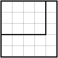
Call the part of boundary of the region bordering the rest of the puzzle the open boundary, and the part on the edge of the puzzle the closed boundary. We need to define the unshaded graph, and count the cycles in it. The main problem is how we’re going to deal with the world outside the region. Let’s assume everything outside the region is connected, so the region isn’t required for connectivity. We can model this by placing a single vertex for the exterior, which every cell on the boundary of the region has an edge to:

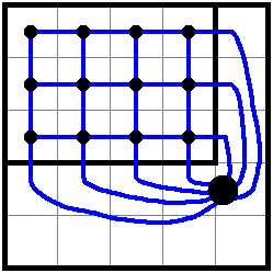
How many cycles does this graph have? Let’s draw them in red:

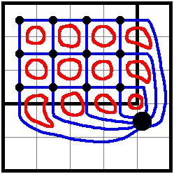
There’s still one cycle per $+$ intersection in the region, as long as we count those on the open boundary. This is easy to count, at least for rectangles: in our example, the $+$ intersections make a 3 by 4 rectangle, so there are 12 cycles.

Placing blocks reduces the number of cycles exactly as before. Specifically, a block in the region which has $b$ sides on the boundary of the puzzle reduces the number of cycles by $3-b$. Note that a side of a block being on the open boundary does not contribute towards $b$.

So we have exactly the same formula as before: if $F$ is the final number of cycles, $I$ is the initial number of cycles, $n$ is the number of blocks in the region, and $b$ is the number of sides of blocks on the closed boundary,$$F=I+b-3n.$$

We need to be somewhat careful in counting cycles in the final unshaded graph. Cycles internal to the region work how you expect, but some cycles go through the outside world.

A cycle that contains the outside world vertex looks a bit different: it’s a path of unshaded cells from one boundary of the region to another. We call this kind of cycle a half-loop. If the outside world is entirely unshaded, a half-loop corresponds to an actual cycle that passes through the region. But half-loops don’t always correspond to actual unshaded cycles, because the outside world may be disconnected by some shaded cells.

It’s often useful to count half-loops separately from internal cycles, e.g. if you can prove there must be a half-loop but don’t yet know where it is. There are some important observations to know about half-loops:

• Two adjacent unshaded cells on the open boundary form a half-loop.
• A single unshaded cell at the corner of the open boundary (so two of its sides border the rest of the puzzle) is a half-loop.
• If the unshaded cells outside the region are disconnected, there must be half-loops to make the unshaded graph connected. In particular, if there are $k$ connected components of unshaded cells in the outside world, there must be at least $k-1$ half-loops.
• If there’s a shaded cell touching the open boundary outside the region, there must be a half-loop starting at the unshaded cell in the region next to that shaded cell.

The last of these is because that unshaded cell needs to be connected to the outside world. A nice way to think about this is to imagine that shaded cells have slivers cut out of each side, or that instead of shading the whole cell you just draw an X. Then the sliver adjacent to the region is an entire unshaded connected component of the outside world, and this is a special case of the previous point.

Example 5

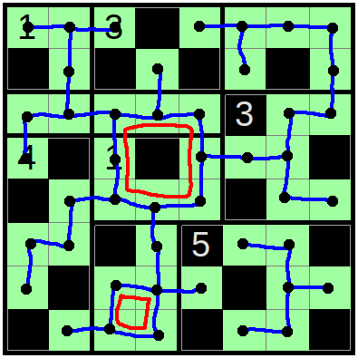
Let’s try using regional cycle counting to solve this puzzle.

How do we know which region to apply cycle counting to? This can be hard to determine. Just like cycle counting on the whole puzzle, regional cycle counting is most effective when there are few spare points, so we can make use of the fact that there are very few cycles. Sometimes you have to try several regions before finding one that’s close enough to maximal for regional cycle counting to be useful.

In this case, we can use the region in the bottom left containing the 13, 4, and 2 rooms.. We need to count the initial cycles, or equivalently count the grid line intersections, including those on the open boundary. The easiest way for me is to think of them as in a $8\times7$ grid, except that $1\times3$ in the top right are missing (because they’re outside the region). So we have $I=8\cdot7-3=53$ cycles.

We can fit 4 blocks on the left and 4 blocks on the bottom, so let’s take a loan for $B=8$. Now we have 61 points, and need to spend 57 of them placing the 19 required blocks. That leaves 4 points to spare.

We need to make a bit of progress to determine where we spend these 4 points. Standard heyawake deductions get us to this point. Now we need to recall the conditions above that force half-loops. In particular, there are two blocks adjacent to the region, which force two half-loops, and the outside world is divided into three connected components, which forces two more.

Alternatively, we can imagine that shaded cells have unshaded slivers on each side. Then our progress so far divides the outside world into five components:

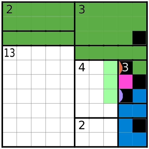
The orange and lavender regions are each just a sliver of a shaded cell; in the previous paragraph we counted the half-loops forced by these shaded cells in a different way. Since there are five outside sections that all need to be connected, there must be four half-loops in our region connecting them.

Whichever way you count, we have shown there must be four half-loops, which is where we spend our remaining four points. We then know

1. We need to pay our debt in full, so the left and bottom edge must each have four blocks.
2. There are no cycles inside the region.
3. There are no more blocks adjacent to the region.
4. There are no more connected components of the outside world: in particular, the large component at the top (colored green above) must be connected on its own, without going through the region.
5. There are no half-loops with both ends on the same component of the outside world.

Just (1) and (3) get us here, and then (5), (2), and standard deductions get us all this. There’s only one way to finish the 13 room. Leaving R9C6 unshaded would make a large half-loop that we can’t afford, so it’s shaded, and the puzzle resolves.

Eccentric exteriors

An additional complexity, which I haven’t seen in many puzzles, arises when the puzzle outside the region isn’t simply connected. For instance, let’s try to use regional cycle counting on this example, where the region crosses the puzzle:

Suppose this is the solution to the puzzle⁷:

Let’s count cycles and see what we find. Initially there are $I=16$ cycles. We place 6 blocks, with 2 on edges, for a cost of $3\cdot6-2=16$. And there’s one half-loop, which crosses the region vertically. It seems like we started with 16 points, and spent 17. What’s going on?

The answer is that the thing I called a half-loop, which connects two different components of the outside world, doesn’t actually form a cycle. You can draw what remains of the graph above after placing all of these blocks, and you’ll see that there are no cycles.

However, this half-loop does reduce the number of connected components, since it connects to otherwise disconnected parts of the outside world. Again we see connected components act like negative cycles: a half-loop either decreases the number of components by 1, or increases the number of cycles by 1.

My preferred way to deal with this case is to say that each additional connected component of the outside world provides 1 point. We will generally have to spend this point on a half-loop connected the components of the outside world together.

Alternatively, you could consider the initial graph (drawn above) to have the outside world merged into one component, or equivalently add an edge between the two components as drawn, even though it has multiple components in the puzzle. This introduces another cycle, which also earns 1 point. This cycle is not obvious because it doesn’t correspond to any intersection of grid lines, like all the other cycles we’ve counted.

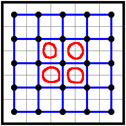
There’s another way the outside world can fail to be simply connected. Let’s use cycle counting on a region which is entirely enclosed in the puzzle, like this:

If you count grid line intersections, you will conclude that there are 16 cycles, but there are actually only 15! Because the outside world goes all the way around the region, the 16 obvious cycles aren’t actually independent. As a result, there will be one less cycle after solving the puzzle than you might have expected.

Here my preferred approach for handling this case. The thick black line represents the outside world, and we connect all the cells touching the outside world to it.

Drawing earlier examples this way would have just elongated the black circle vertex representing the outside world, without changing the structure of the graph. But now the outside world isn’t contractible; a single vertex isn’t able to represent the structure it has. With this representation, there are initially 16 cycles as expected. But after solving the puzzle, there must still be at least one cycle, namely the one in the outside world going all the way around the region, which we must spend a point on.

To make this more explicit, suppose the solution looks like this:

We’ve spent 15 of our 16 points placing those 5 blocks. What’s left of the graph is essentially just the loop of the outside world that goes around the region. We have to give up our final point to pay for this loop.

To summarize the adjustments needed when the outside world isn’t simply connected:

• For each additional connected component of the outside world, we earn 1 point.
• For each cycle in the outside world, we must pay 1 point.

Example 6

Here’s a puzzle for you to practice cycle counting on a weird region.

I won’t go through this one in detail, but to get you started in case you’re stuck: use cycle counting on this region. If you count correctly using the naive loan of $B=10$, you should find that you have 132 points (2 of which are from the outside world having three components), of which 129 need to be spent placing blocks and 2 need to be spent connecting the components of the outside world. It’s possible you’ll find another region which also succumbs to cycle counting.

Example 7

Here another large puzzle, that involves counting cycles in another weird-shaped region.

I suggest using cycle counting on the $13\times10$ rectangle in the center. You should find that you have 154 total points, and need to spend one on the cycle of the outside world and 150 on placing blocks.

That still leaves 3 points; here’s my argument for how they have to be spent: first, the left and right edges have even length, so they must each either have an unshaded cell in a corner or two adjacent unshaded cells, either of which is a half-loop. For the final point, note that the two 1 regions force us to shade cells on opposite parity (meaning the color of the cell if you checkerboard the grid). Blocks can only be diagonally connected to blocks of the same parity, so there must be two separate groups of blocks that aren’t connected to each other. That means there’s a path of unshaded cells separating the two groups, which is a half-loop we have to spend our last point on.

The most general formula

Let’s directly derive a cycle counting formula which works for any shape of puzzle and region. This will get a bit more mathy. We’ll rely on the following fact, which isn’t hard to prove (e.g. using the definition of $\bar\chi$ and inclusion-exclusion).

Fact. Let $A$ and $B$ be graphs, possibly sharing some vertices. Then$$\bar\chi(A\cup B)=\bar\chi(A)+\bar\chi(B)-\bar\chi(A\cap B).$$

The union or intersection of graphs $A$ and $B$ is just the graph obtained by taking the union or intersection of the vertices and edges separately.

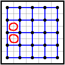
We want to use cycle counting on some region. Let $G$ be the graph of unshaded cells in the region, including an extra vertex for each cell on the boundary to represent that connection to the outside world. Let $W$ be the graph representing the outside world: $W$’s vertices are these extra vertices, and $W$ has edges connecting them according to the shape of the puzzle. Choose $G$ and $W$ so that they do not share any edges.

For instance, to do regional cycle counting on this region, I would choose $G$ to be (what will remain after shading cells of) the blue graph and $W$ to be the purple graph. Note that $G$ includes vertices just outside the region, $G$ and $W$ share several vertices (but no edges), and $W$ only includes the immediate vicinity of the region, not the whole puzzle since otherwise it would have lots of cycles that I don’t want to think about.

What does the fact above tell us? Recall that $\bar\chi(G)=E-V+1=\operatorname{cyc}(G)-\operatorname{cmp}(G)+1$. Since the unshaded cells have to be connected, $\bar\chi(G\cup W)$ is the number of cycles in the final graph, which we’ve been calling $F$.

So we have$$F=\operatorname{cyc}(G)-\operatorname{cmp}(G)+1+\bar\chi(W)-E(G\cap W)+V(G\cap W)-1.$$

Since $G$ and $W$ share no edges, $E(G\cap W)=0$. Rearranging,$$F=\operatorname{cyc}(G)+(V(G\cap W)-\operatorname{cmp}(G))+\bar\chi(W).$$

The most confusing term here is the middle one, $V(G\cap W)-\operatorname{cmp}(G)$. I claim this is just the number of half-loops! By connectivity, each connected component of $G$ must touch the boundary, meaning it includes some vertex in $G\cap W$. A half-loop is when two of these vertices are in the same component of $G$. If there are no half-loops, $V(G\cap W)=\operatorname{cmp}(G)$, and each half-loop decreases $\operatorname{cmp}(G)$ by one, so the difference counts the half-loops.

We can expand $\bar\chi(W) = \operatorname{cyc}(W)-(\operatorname{cmp}(W)-1)$. This captures what we saw in the previous section: a cycle in $W$ costs a point, and an extra connected component of $W$ provides a point.

Finally, we know from before that $F=I-3n+b$, where we start with $I$ cycles, and each block removes three cycles unless it’s on the boundary of the puzzle, which happens $b$ times. So to conclude:

Theorem. To perform cycle counting on a region, let $G$ be the unshaded graph of the region including its boundary, and let $W$ be a graph representing the outside world, as described above. Then$$I-3n+b=\operatorname{cyc}(G) + \text{\# half-loops} + \operatorname{cyc}(W) - (\operatorname{cmp}(W)-1),$$where $I$ is the initial number of cycles in the initial graph including the outside world, $n$ is the number of shaded cells in the region, and $b$ is the number of edges of those shaded cells touching the boundary of the puzzle.

Rearranging to the form I find easiest to use, where $B$ is an upper bound on the number of edges of blocks in the region on the boundary of the puzzle, we have $$I + B +(\operatorname{cmp}(W)-1) = 3n + (B-b) + \operatorname{cyc}(G) + \text{\# half-loops} + \operatorname{cyc}(W).$$ In words:

We earn (left-hand side)

• 1 point from each cycle in the initial graph (including the outside world)
• $B$ points from our loan, by promising to place $B$ blocks on the boundary of the puzzle
• 1 point from each connected component of the outside world past the first.

We spend (right-hand side)

• 3 points for each block we place
• $B-b$ points for failing to meet the promise we made for our loan
• 1 point for each cycle in the region (after solving the puzzle)
• 1 point for each half-loop
• 1 point for each cycle in the outside world.

This formula even works when the region is disconnected: $I$ counts the number of cycles in the initial graph including the outside world, which essentially means you should just add the number of cycles in each connected component of the region (and account for the adjustments based on the shape of the outside world). So this is basically just using cycle counting on each component separately, and adding the results. It might be useful if you can prove that there’s a cycle in some component but can’t determine which: for instance, a chain of blocks that splits the outside world still forces there to be a half-loop, though it might be in either component that the chain goes between.

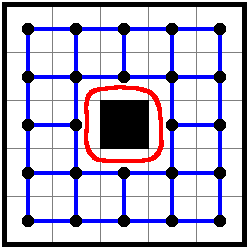
In our simple example, after shading some cells, the graphs look like this:

Now $G$ has 12 components (8 of which are individual vertices outside the region), and $G\cap W$ consists of the 12 boundary vertices, so the number of half-loops is $V(G\cap W)-\operatorname{cmp}(G)=0$ (as we expect, since there don’t appear to be any half-loops). It’s not hard to compute the rest of the variables, and check that they satisfy the equation (with no loan $B=0$) $$16 + 0 + (1-1) = 3\cdot 5 + (0-0) + 0 + (12-12) + 1.$$

A challenge

Here’s one last puzzle for you. It’s on a torus: opposite edges of the boundary are merged, for the purposes of unshaded connectivity, no adjacent blocks, and the heyawake rule. No rooms extend past the edge of the grid.

You’ll need to be careful when counting cycles, since it works a bit differently on a torus, though the relevant general equations still hold. In case you prefer to work on an unrolled torus, here’s a grid with 9 copies of the puzzle.

---

1. There are also penalty theories for other types of puzzles, but this post only considers dynasty penalty theory. ↩

2. All puzzles in this post are my own. ↩

3. Either of these usually adds one cycle. ↩

4. Really we want the dimension of the cycle space, and the interior faces give a convenient basis. ↩

5. Actually the negative of this expression, but that’s an arbitrary convention and I’ll use this one instead because it’s more convenient. ↩

6. This is shorthand for the cell in row 10, column 6, counting from the top left. ↩

7. This violates the heyawake rule, but that doesn’t affect what I’m trying to illustrate. ↩